Accuracy of models using Lenskit

This notebook shows how to test the recommendations accuracy of models using lenskit.

Setup

from lenskit.datasets import MovieLens
from lenskit import batch, topn, util
from lenskit import crossfold as xf
from lenskit.algorithms import Recommender, als, item_knn, basic
import lenskit.metrics.predict as pm
import pandas as pd

/Users/carlos/anaconda3/lib/python3.7/site-packages/fastparquet/encoding.py:222: NumbaDeprecationWarning: The 'numba.jitclass' decorator has moved to 'numba.experimental.jitclass' to better reflect the experimental nature of the functionality. Please update your imports to accommodate this change and see http://numba.pydata.org/numba-doc/latest/reference/deprecation.html#change-of-jitclass-location for the time frame.
  Numpy8 = numba.jitclass(spec8)(NumpyIO)
/Users/carlos/anaconda3/lib/python3.7/site-packages/fastparquet/encoding.py:224: NumbaDeprecationWarning: The 'numba.jitclass' decorator has moved to 'numba.experimental.jitclass' to better reflect the experimental nature of the functionality. Please update your imports to accommodate this change and see http://numba.pydata.org/numba-doc/latest/reference/deprecation.html#change-of-jitclass-location for the time frame.
  Numpy32 = numba.jitclass(spec32)(NumpyIO)
/Users/carlos/anaconda3/lib/python3.7/site-packages/fastparquet/dataframe.py:5: FutureWarning: pandas.core.index is deprecated and will be removed in a future version.  The public classes are available in the top-level namespace.
  from pandas.core.index import CategoricalIndex, RangeIndex, Index, MultiIndex

Load data

mlens = MovieLens('data/ml-latest-small')
ratings = mlens.ratings
ratings.head()

	user	item	rating	timestamp
0	1	31	2.5	1260759144
1	1	1029	3.0	1260759179
2	1	1061	3.0	1260759182
3	1	1129	2.0	1260759185
4	1	1172	4.0	1260759205

Define algorithms

biasedmf = als.BiasedMF(50)
bias = basic.Bias()
itemitem = item_knn.ItemItem(20)

Evaluate recommendations

def create_recs(name, algo, train, test):
    fittable = util.clone(algo)
    fittable = Recommender.adapt(fittable)
    fittable.fit(train)
    users = test.user.unique()
    # now we run the recommender
    recs = batch.recommend(fittable, users, 100)
    # add the algorithm name for analyzability
    recs['Algorithm'] = name
    return recs

We loop over the data to generate recommendations for the defined algorithms.

all_recs = []
test_data = []
for train, test in xf.partition_users(ratings[['user', 'item', 'rating']], 5, xf.SampleFrac(0.2)):
    test_data.append(test)
    all_recs.append(create_recs('ItemItem', itemitem, train, test))
    all_recs.append(create_recs('BiasedMF', biasedmf, train, test))
    all_recs.append(create_recs('Bias', bias, train, test))

We create a single data frame with the recommendations

all_recs = pd.concat(all_recs, ignore_index=True)
all_recs.head()

	item	score	user	rank	Algorithm
0	3171	5.366279	9	1	ItemItem
1	104283	5.279667	9	2	ItemItem
2	27803	5.105468	9	3	ItemItem
3	4338	5.037831	9	4	ItemItem
4	86000	4.991602	9	5	ItemItem

We also concatenate the test data

test_data = pd.concat(test_data, ignore_index=True)

Let’s analyse the recommendation lists

rla = topn.RecListAnalysis()
rla.add_metric(topn.ndcg)
results = rla.compute(all_recs, test_data)
results.head()

		nrecs	ndcg
Algorithm	user
Bias	1	100.0	0.0
	2	100.0	0.0
	3	100.0	0.0
	4	100.0	0.0
	5	100.0	0.0

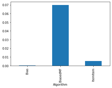
Let’s see the nDCG mean value for each algorithm

results.groupby('Algorithm').ndcg.mean()

Algorithm
Bias        0.000309
BiasedMF    0.069957
ItemItem    0.005367
Name: ndcg, dtype: float64

results.groupby('Algorithm').ndcg.mean().plot.bar()

<matplotlib.axes._subplots.AxesSubplot at 0x12335b110>

Evaluate prediction accuracy

def evaluate_predictions(name, algo, train, test):
    algo_cloned = util.clone(algo)
    algo_cloned.fit(train)
    return test.assign(preds=algo_cloned.predict(test), algo=name)

preds_bias = pd.concat(evaluate_predictions('bias', bias, train, test) for (train, test) in xf.partition_users(ratings, 5, xf.SampleFrac(0.2)))
preds_biasedmf = pd.concat(evaluate_predictions('biasedmf', biasedmf, train, test) for (train, test) in xf.partition_users(ratings, 5, xf.SampleFrac(0.2)))
preds_itemitem = pd.concat(evaluate_predictions('itemitem', itemitem, train, test) for (train, test) in xf.partition_users(ratings, 5, xf.SampleFrac(0.2)))

Bias

print(f'MAE: {pm.mae(preds_bias.preds, preds_bias.rating)}')
print(f'RMSE: {pm.rmse(preds_bias.preds, preds_bias.rating)}')

MAE: 0.6950106667260073
RMSE: 0.9066546007561017

BiasedMF

print(f'MAE: {pm.mae(preds_biasedmf.preds, preds_biasedmf.rating)}')
print(f'RMSE: {pm.rmse(preds_biasedmf.preds, preds_biasedmf.rating)}')

MAE: 0.6818618886318303
RMSE: 0.8911595961607526

ItemItem

print(f'MAE: {pm.mae(preds_itemitem.preds, preds_itemitem.rating)}')
print(f'RMSE: {pm.rmse(preds_itemitem.preds, preds_itemitem.rating)}')

MAE: 0.6640965754633255
RMSE: 0.8730680515165724